Lotka Volterra model [Useful for competitive exams’24 of Life Science]

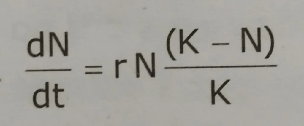
The Lotka Volterra model of interspecific competition is a simple mathematical model representing the interaction between two competing species. This mathematical model was developed by two people working independently -Alfred Lotka (1925), an insurance actuary, and Vito Volterra (1926) a mathematical physicist. One the basis of this model, the losers of the competitive interactions can be predicted. The Lotka-Volterra equation for interspecific competition is based on the Verhulst-Pearl logistic growth equation:

The logistic equation and Lotka Volterra model equations for two species (species 1 and species 2).

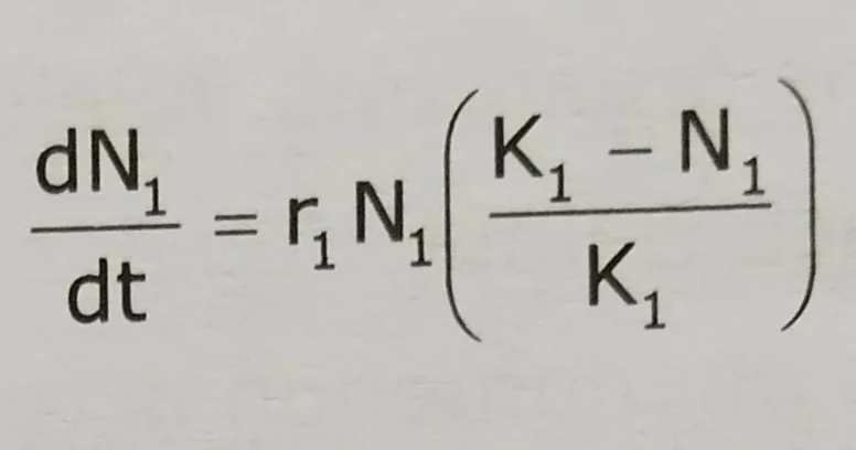
The logistic equation for species 1 growing alone:

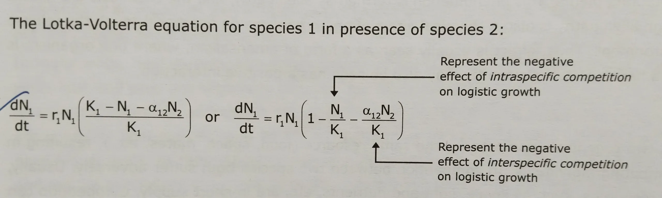
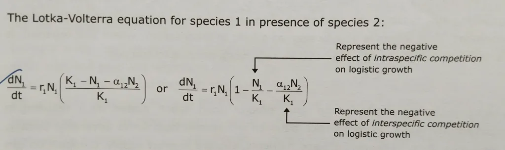
The Lotka Volterra model equation for species 1 in the presence of species 2:

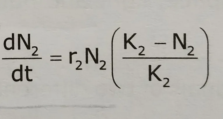
The logistic equation for species 2 growing alone:

The Lotka Volterra model equation for species 2 in the presence of species 1:

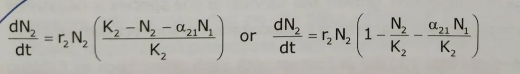
Where N1 and N2 = population of species 1 and 2, respectively

K1 and K2 = carrying capacity of system for each species in the absence of the other.
t= time
r1 and r2= intrinsic rate of increase of species 1 and species 2, respectively

α₁₂= is a competition coefficient representing the effect of one individual of species 2 on the growth of species 1

α₂₁= is a competition coefficient representing the effect of one individual of species 1 on the growth of species 2

The explanation of Lotka Volterra Model:

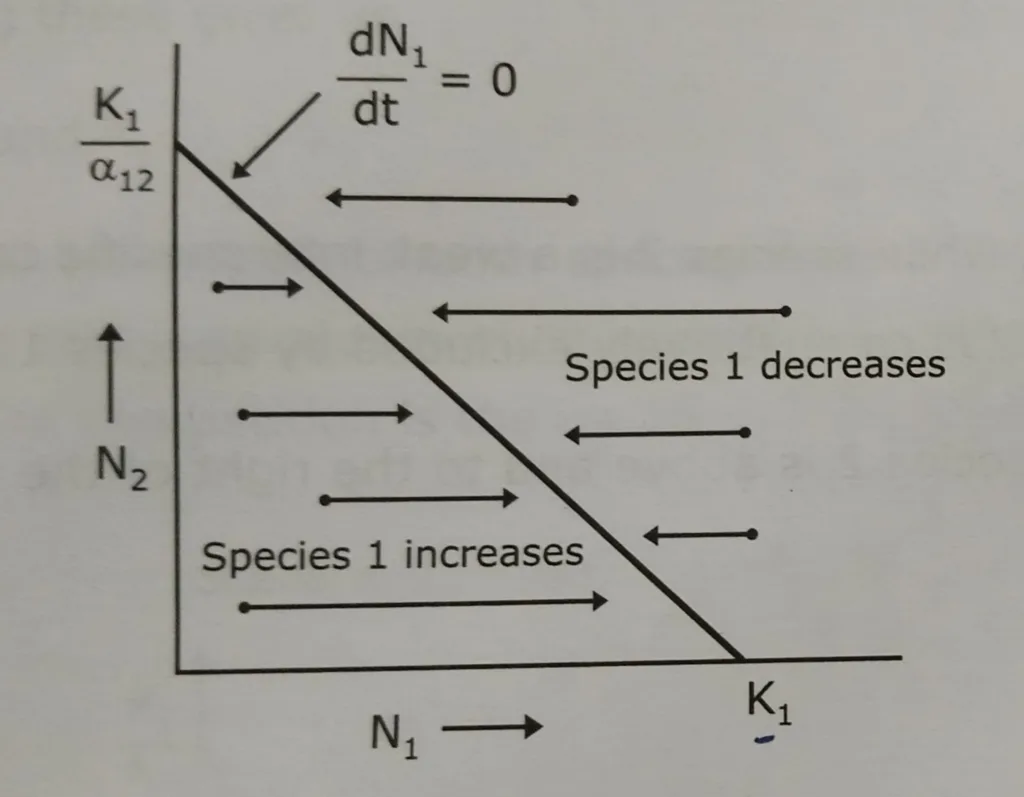
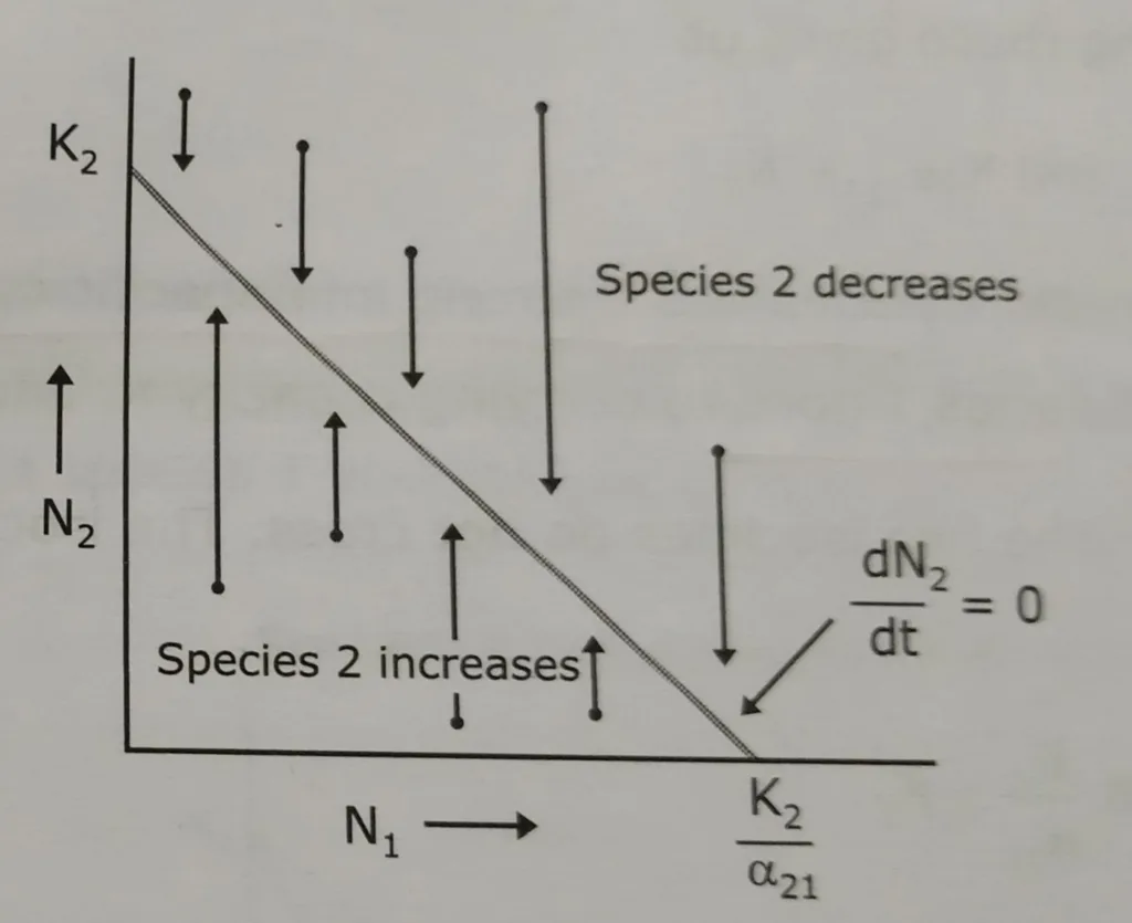
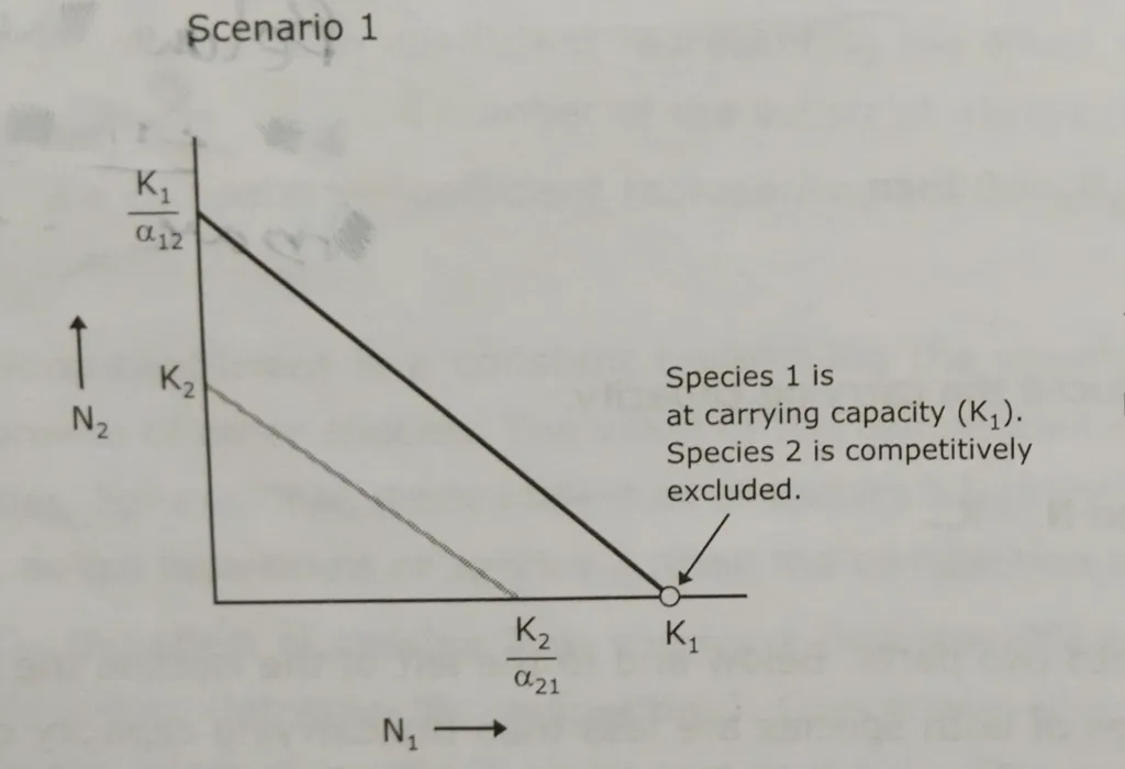
To understand the predictions of the model it is helpful to look at graphs that show how the size of each population increases or decreases when we start with different combinations of species abundances. These graphs are called state-space graphs, in which the population size of species 1 is plotted on the X-axis, and the population size of species 2 is plotted on the Y-axis. Each point in a state-space graphs represents a combination of abundances of the two species. For each species there is a straight line on the graph called a zero isocline.

The zero isocline for each species states that at any given point along that line the population size does not change, i.e. dN/dt= 0. The two graphs show the zero isocline for species 1 and species 2. Any point above the zero isocline indicates that the population of that species is decreasing; any point below the isocline that population is increasing.

Scenarios of the Lotka Volterra model

The two zero isoclines can be juxtaposed in four different ways, depending on the relative values of α and K for each species.

The four possible competitive situations, defined by the relative positions of the isoclines, are given below.

Scenario 1:

The two isoclines do not cross. The isocline of species 1 is above and to the right of the right of the isocline for species 2.

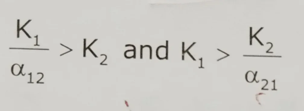
Rearranging these given us

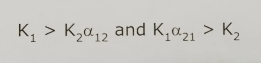
In this scenario, species 1 is a strong interspecific competitor, while species 2 is a weak interspecific competitor.

Outcome:
Species 1 goes to carrying capacity K1 and species 2 is competitively excluded by species 1.

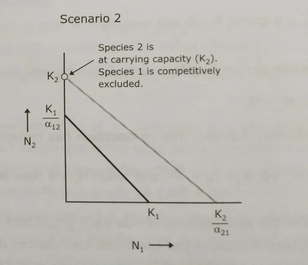
Scenario 2:

The two isoclines do not cross. The isocline of species 2 is above and to the right of the right of the isocline for species 1.

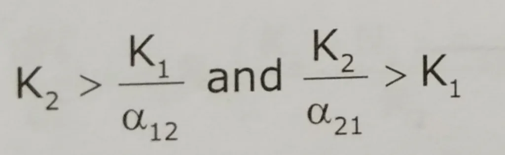
Rearranging these given us

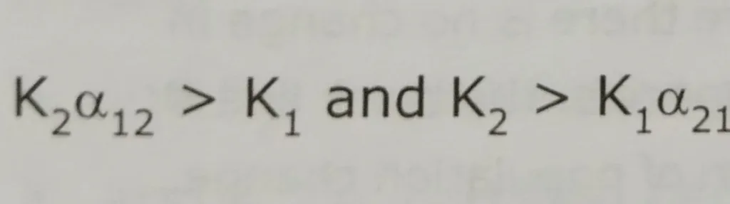
In this scenario, species 2 is a strong interspecific competitor, while species 1 is a weak interspecific competitor.

Outcome:
Species 2 goes to carrying capacity K2 and species 2 is competitively excluded by species 3.

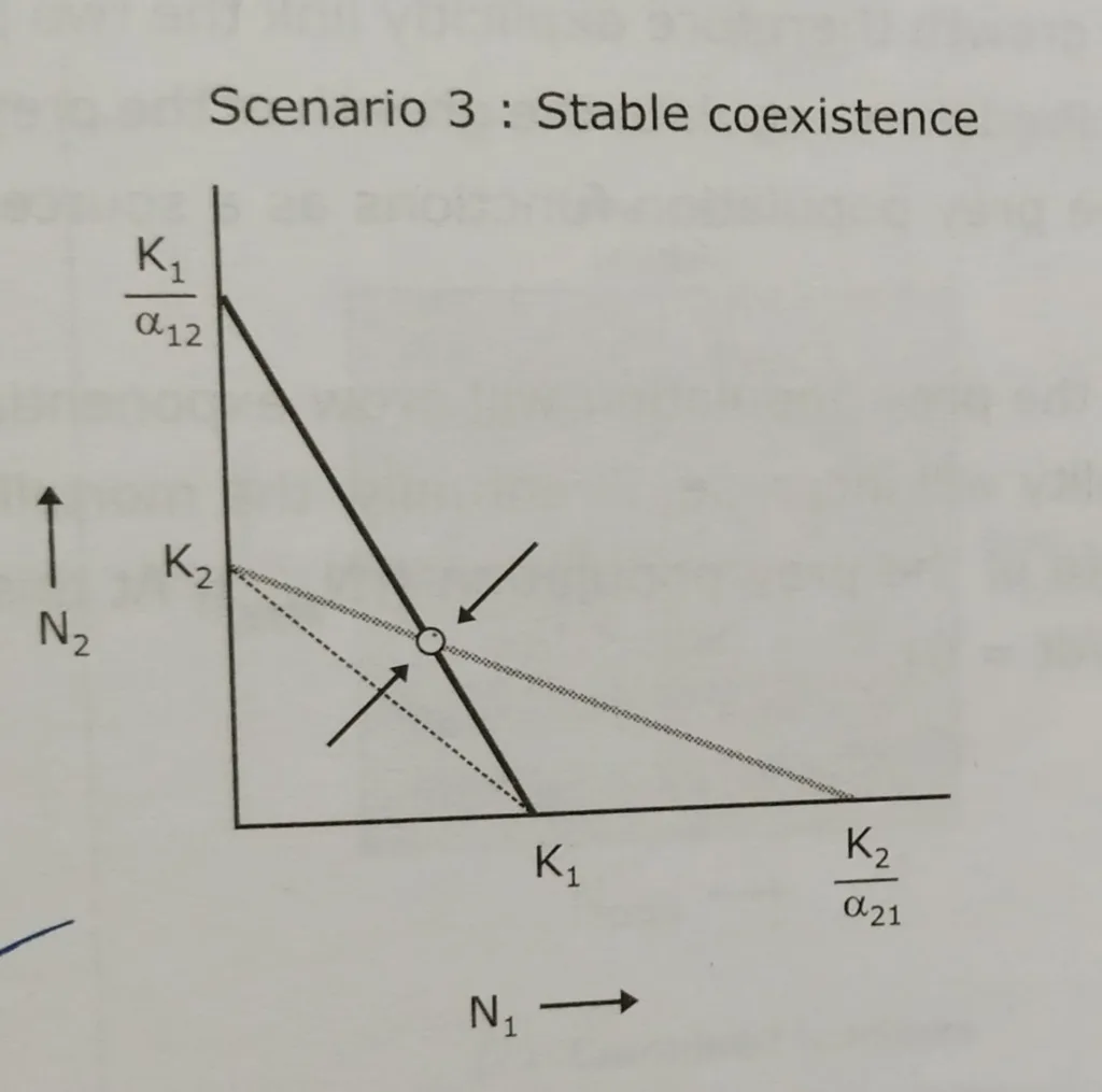
Scenario 3:

The case of stable coexistence

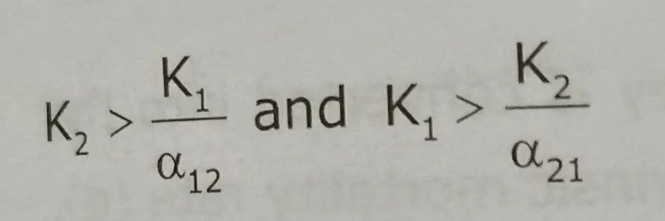
The isoclines cross one another, but for both species carrying capacities are lower than the other’s carrying capacity divided by the competition coefficient. Rather than outcompeting one another, the two species are able to coexist at stable equilibrium point. An equilibrium point occurs where the isoclines cross.

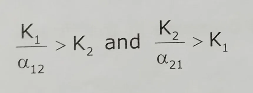
Rearranging these given us

In this case, both species have less competitive effect on each other. i.e. weak interspecific competition. Coexistence occurs when interspecific competition is greater than interspecific competition. The outcome of this type of competition is the stable coexistence of both species.

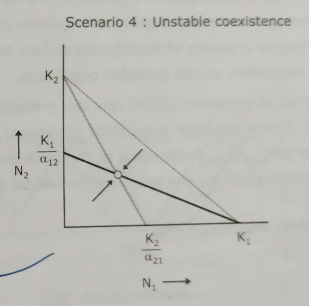
Scenario 4:

The case of unstable coexistence

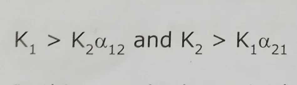
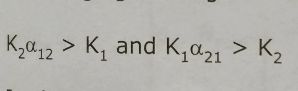
The isoclines of the two species cross one another. Here, the carrying capacity of species 1 (K1) is higher than the carrying capacity of species 2 divided by the competition coefficient (K2/α₂₁), and the carrying capacity of species 2 (K2) is higher than the carrying capacity of species 1 divided by the competition coefficient (K2/α₁₂). There is an unstable equilibrium point where the isoclines intersect.

Rearranging these given us

In this case, individuals of both species have a greater competitive effect on each other. Competitive exclusion occurs when interspecific competition is greater than interspecific competition. The outcome of this type of competition is the unstable coexistence between species 1 and species 2.

Other notes useful for CSIR NET:

1. Photorespiration: https://thebiologyislove.com/photorespiration-or-c2-pathway/
2. Apoptosis Pathway: https://thebiologyislove.com/apoptosis-pathway/
3. Population density: https://thebiologyislove.com/determination-of-population-density/

Facebook link: https://www.facebook.com/share/p/LhRb6Q74D5zPfnoJ/?mibextid=oFDknk

Instagram link: https://www.instagram.com/p/C68_ikipU2X/?igsh=NnNpZ3Joc2h0amE1